The question:
how to control opinions in a social group by creation of an environment with whom the group can interact ?
Let us start to define the toy model.
In a given social group we have a set of opinions $K$ distributed among all group members. The group collaborates with external world through an interaction with some set of opinions stated in an external environment. We assume that the environment is too big to be manipulated by the social group, but the environment can modify somehow the distribution of opinions inside the group.
For a better transparency we consider 2 different opinions described as $A$ and $B$. Opinions $A$ and $B$ are defined as states "+1" and "-1" correspondingly. Members are distributed among two subgroups according to a shared opinion and interact with the same environment but with different strength: $\gamma_{A}$ and $\gamma_{B}$ respectively. The $\gamma_{A|B}$ coefficients correspond to the level of group members acceptance of noise created by the environment. Or, in other words, the coupling constants $\gamma_{A|B}$ are weights which characterize how much a given group relies on opinions supported by the environment. The level of believe in a group is proportional to the value of $\gamma_{i}$ couplings. The scheme is depicted in the picture 1.

fig. 1. The environmental $M$ levels are coupled to 2 separate systems $A$ and $B$ with a given coupling constants $\gamma_{A}$ and $\gamma_{B}$. For simplicity each group $A$ and $B$ has the same number of levels $N$.
We assume that the social model will fulfill the principle of least action so the entire set will tend to minimize the total energy. Therefore the Hamiltonian approach should make a frame for our analysis. The model can be described by the following Hamiltonian: \begin{equation} \label{Hamiltonian0} H = H_{A} + H_{B} + H_{E} + H_{Int} \end{equation} where
\begin{equation} \label{Hamiltonian1} H_{A|B} = \sum_{k_{A|B} = 1}^{N_{A|B}} E_{A|B} \left| A|B_{k_{A|B}} \right> \left< A|B_{k_{A|B}} \right| \end{equation} describes the state of subgroups $A$ and $B$ with energies $E_{A}$ ($E_{A}$) and $N_{A}$ ($N_{A}$) discrete states $\left| A_{k_{A}} \right>$ ($\left| B_{k_{B}} \right>$). \begin{equation} \label{Hamiltonian2} H_{E} = \sum_{n = 1}^{M} E_{n} \left| E_{n} \right> \left< E_{n} \right| \end{equation} is the basic energy of the environment with $M$ discrete states $\left| E_{n} \right>$ labeled by index n. The interaction between the groups and the environment has a form: \begin{equation} \label{Hamiltonian3} H_{Int} = \sum_{n=1}^{M} \left[ \left( \sqrt{ \gamma_{A} } \sum_{ k_{A} = 1}^{ N_{A} } VA_{k_{A}}^{n} \left| A_{k_{A}} \right> \left< E_{n} \right| + h.c. \right) + \left( \sqrt{ \gamma_{B} } \sum_{ k_{B} = 1}^{ N_{B} } VB_{k_{B}}^{n} \left| B_{k_{B}} \right> \left< E_{n} \right| + h.c. \right) \right ] \end{equation} where $VA$ and $VB$ are matrix elements describing couplings between group states $\left| A \right>$, $\left| B \right>$ and environmental levels $\left< E_{n} \right|$.
Because the environment cannot be modified by any group we can use the Markovian approximation and eliminate the environment states from the Hamiltonian above. The result of operation can be written in the following form: \begin{equation} \label{Hamiltonian4} H_{eff} = H_{A} + H_{B} - i V \cdot V^{+} \end{equation} where \begin{equation} \label{Hamiltonian5} V = \left( \begin{array}{} \sqrt{ \gamma_{A} } \cdot VA \\ \sqrt{ \gamma_{B} } \cdot VB \end{array} \right) \end{equation} creates a dissipative part of the effective Hamiltonian $H_{eff}$ which is an $N \times N$ dimensional matrix and matrix $V$ has a dimension $N \times M$ . Our analysis of the dynamics of the system can be reduced to the determination of the eigenvalues of the effective Hamiltonian $H_{eff}$: $\Lambda = x - iy$ which are complex. An imaginary part describes how fast (time $\tau$) a given eigenvalue dissipates in the system: $ \tau \approx \frac{1}{y}$.
In other words, the $\tau$ describes the lifetime of a given opinion values by the real value of the eigenvalue $x$ . Let us stress that we allow to create a continuous number of opinions, not only those which are defined in the assumptions of the issue: $E_{A|B}$ . Why can the eigenvalues of the Hamiltonian be used as a determinant of the social opinion distribution ?
A standard model of opinion evolution is modeled using (in a simplest case) a set of linear equations: \begin{equation} \label{Hamiltonian6} \vec{x} \left( t + 1 \right) = W \vec{x} \left( t \right) \end{equation} where $W$ is some $N\times N$ matrix describing an information exchange with weights between participants of the social network and the vector $\vec{x}$ is an opinion profile in the network calculated for the time $t$. Thus, the correspondence between the opinion profile $\vec{x}\left( t \right)$ and our approach can be done by calculation of a power spectrum of the $\vec{x}\left( t \right)$. Positions of maximums in the power spectrum can be understood as equivalent to the real values of eigenvalues of the Hamiltonian $H_{eff}$ while the time scale of change of the profile $\vec{x}\left( t \right)$ corresponds to the imaginary part of the eigenvalues (to be more specific to the inverse of the imaginary part).
For any numerical calculations we have to define values $M$, $N$, $E_{A}$, $E_{B}$, $N_{A}$, $N_{B}$, $\gamma_{A}$, $\gamma_{B}$. The matrices $VA$ and $VB$ are calculated as Gaussian unitary ensembles (GUE random matrices).
Below we present a variety of plots of numerically determined eigenvalues of the Hamiltonian.
On all plots the dots are a result of numerical calculations of the Hamiltonian $H_{eff}$. Numerical simulations have been done for 30 GUE matrices $V$ with $N = 100$ and $M = 60$. Remaining values of parameters used for simulations:
- energies: $E_{A} = -1/2$, $E_{B} = 1/2$,
- number of states: for state $A$: $N_{A} = 50$, for state $B$: $N_{B}=50$,
- interaction couplings are described for each plot separately.
At the beginning, for a comparison with existing models we shows on Fig. 2,3 and 4 a situation where $\gamma_{A} = \gamma_{B}$ and different values of $\gamma_{B}$. A similar plots one can find in the work [1].
For a better visibility we used for scale $y$ logarithmic scale. In our case $y \leftarrow -log( \left| y \right| )$, so the value $y=-3$ corresponds to $y = 10^{-3}$.

Fig. 2. Simulation for $\gamma_{A} = \gamma_{B} = 0.0025$ in energy units. The left vertical plot shows the integrated density profile of the width of calculated eigenvalues. The upper picture presents the integrated spectral density showing the width of energy states.

Fig. 3. Simulation for $\gamma_{A} = \gamma_{B} = 0.01$. An creation of two timescales of the eigenvectors is visible.

Fig. 4. Simulation for $\gamma_{A} = \gamma_{B} = 0.5$.
The next Figs (5,6,7 and 8) shows asymmetric situations where $\gamma_{A} = \gamma_{B}/10$ and different values of $\gamma_{B}$. Detailed values of other parameters are noted in the figure description.

Fig. 5. The situation with $\gamma_{B} = 0.01$ and $\gamma_{A} = \gamma_{B}/10$.

Fig. 6. The eigenvalue spectrum calculated for $\gamma_{B} = 0.05$ and $\gamma_{A} = \gamma_{B}/10$.

Fig. 7. The spectrum calculated for $\gamma_{B} = 0.1$ and $\gamma_{A} = \gamma_{B}/10$.
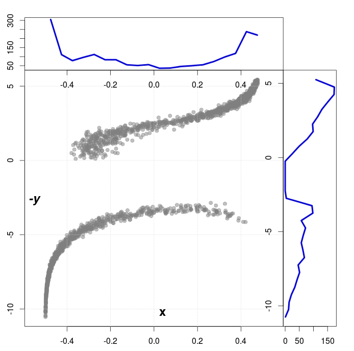
Fig. 8. The spectrum calculated for $\gamma_{B} = 0.5$ and $\gamma_{A} = \gamma_{B}/10$.
Conclusions
The landscape presented on all plots of eigenvalues of the Hamiltonian $H_{eff}$ is quite straightforward for those who are familiar with atomic physics, especially interactions of multi-level atomic transitions with resonant light. We see clear existence of so called coupled and uncoupled level (states) combinations . The increase of the coupling constant $\gamma_{A|B}$ leads to a creation of grouping of eigenvalues.
The eigenfunctions in the Hamiltonian can be formed in such a way that some combinations of levels cancel the interaction part with the environment - they are called uncoupled (or trapped) states. The number of such states is $N-M$.
Other level eigenfunctions are coupled with the environment's states - such an eigenfunction we call coupled (or un-trapped) states ($M$ decaying states). Populations of trapped states can survive longer time (smaller values of y) in comparison to the un-trapped states, where the populations is exchanged between coupled states by the interaction term proportional to $\sqrt{\gamma_{A|B}}$.
Let us try to translate this physical picture into a social language.
- The coupled (un-trapped) states: configurations of members (eigenfunction) which change a common opinion (eigenvalue) faster due to the interaction with a noisy environment represented by a different set of environmental opinions. Such an exchange of opinion is proportional to the interaction strength $\gamma_{i}$ ($i=A|B$).
- The uncoupled (trapped) states: ideally, such configurations of members (eigenfunction) which create a stable combinations of a group members. They do not interact with the environment.
A higher level of noise (larger value of $\gamma_{A|B}$ and different values of couplings $\gamma_{A} < \gamma_{B}$) doesn't lead to reduction of a significance of unwanted opinions but creates just the opposite action:
it sharpens the polarization of existing opinions and increases the importance of resistance against the environment in a society. Such a situation can be well identified nowadays. The noisy environment is created by mainstream media. What one can find in such an environment: an increasing number of different subjects, news focused on accidents, preferred shorter forms and propagation of a number of opposite opinions and many other similar, as well as different ways of distraction of reader's attention.
Groups of people strongly coupled to such a media stream are not able to define a private opinion and they are easy to manipulate. It also means that the number of people in such a chaotic environment will migrate rather to more stable social groups (trapped states), not so strongly dominated by the mainstream news.
The creation of people without a strong, private opinions is a goal of the present liberal governments. But, as it is presented in this note the chosen way of social control leads just to opposite behaviour. You can see it around yourself, don't you ?
In the model, we used the condition where the number of intermediate states in the environment $M$ is smaller that the number of states in considered social groups $N$: $M < N$.
The opposite case leads to a bit different picture than described in this note, but it is a subject for an another post.
Bogdan Lobodzinski
Data Analytics For All Consulting Service
References:
- E.Gudowska-Nowak, G. Papp and J. Brickmann, Two-Level System with Noise: Blue's Function Approach, Chem. Phys., 220 120-135 (1997)