Sell - buy signals for financial instruments - a multivariate survival analysis approach (in R).

Survival analysis could be understand as a kind of a forecasting method created for studying how long an analyzed subject will exist. In a survival framework we calculate survival probability of a thing at particular points of time.
And so, it is a natural choice to use the survival method in forecasting of financial market. Especially, for prediction of future price behaviour of a given financial instance and as a consequence for generating buy-sell signals. Searching for some examples of similar analysis I have found only a single work addressing the subject [1]. From this publication I adopted a definition of a daily revenue - given below.

In this note I would like to show how to use the survival analysis method for generation of buy/sell signals for a chosen financial product. As data I use Brent Oil Future options, however the method could be adopted to other instruments as well.

The analysis is presented in R language.
As an input I use historical data of Brent Oil Future options available on the portal stooq.pl. The data contain several features like Open and Close prices, Volume, highest (High) and lowest (Low) prices and Open Interest (OpenInt). Operating on a daily basis, my goal is to predict whether for the next day we expect increase or decrease of the Close value.
Let me begin with preparation of libraries and data engineering.

set.seed(1)
library(ggplot2)
library(lubridate)
library(readr)
library(MASS)
library(survival)
library(xts)
library(rms)

# reading the data:
myDir <- "/analysis/forecasting/data_stooq.pl/"
myFile <- "sc_f_d_2015_2016.csv" 
input <- NULL
input <- read.csv(paste(myDir,myFile,sep=""),header=TRUE)

names(input)
[1] "Date"          "Open"          "High"          "Low"           
[5]"Close"         "Volume"        "OpenInt"

In a next step I will introduce new features:

1. $corp = Close - Open$ : it corresponds to the definition of the corp of the candlesticks,

   input$corp <- 0 
   input$corp <- input$Close - input$Open

2. Exponential Moving Average - $EMAV$. For this purpose I use functions for calculation of the Volume Weighted Exponential Moving Average (see volume-weighted-exponential-moving-average)

   VEMA.num <- function(x, volumes, ratio) {
           ret <- c()
           s <- 0
           for(i in 1:length(x)) { 
               s <- ratio * s + (1-ratio) * x[i] * volumes[i];
               ret <- c(ret, s); 
           }
           ret
   }
   
   VEMA.den <- function(volumes, ratio) {
           ret <- c()
           s <- 0
           for(i in 1:length(x)) { 
               s <- ratio * s + (1-ratio) * volumes[i]; 
               ret <- c(ret, s); 
           }
           ret
   }
   
   VEMA <- function(x, volumes, n = 10, wilder = F, ratio = NULL, ...)
   {
           x <- try.xts(x, error = as.matrix)
           if (n < 1 || n > NROW(x))
                   stop("Invalid 'n'")
           if (any(nNonNA <- n > colSums(!is.na(x))))
                   stop("n > number of non-NA values in column(s) ", 
                   paste(which(nNonNA),collapse = ", "))
           x.na <- xts:::naCheck(x, n)
           if (missing(n) & !missing(ratio)) {
                   n <- trunc(2/ratio - 1)
           }    
           if (is.null(ratio)) {
                   if (wilder)
                           ratio <- 1/n
                   else ratio <- 2/(n + 1)
           }
           
           foo <- cbind(x[,1], volumes, VEMA.num(as.numeric(x[,1]), volumes, ratio), 
                        VEMA.den(volumes, ratio))
           (foo[,3] / foo[,4]) -> ma
           
           ma <- reclass(ma, x)
           if (!is.null(dim(ma))) {
                   colnames(ma) <- paste(colnames(x), "VEMA", n, sep = ".")
           }
           return(ma)
   }
   
   x <- ts(input$Close)
   input$EMAV <- 0
   Vol <- rep(1, length(input[,1]))   
   input$EMAV <- VEMA(input$Close, Vol,ratio=0.95)
   plot(input$Close,type="l");lines(input$EMAV,col="red")

3. Daily Revenue - $DailyRevenue$ . The feature is calculated as a percentage of $Close$ values between present and previous days [1]
   $DailyRevenue = \frac{( Close[k] - Close[k-1] )}{Close[k-1]} \cdot 100$

   input$DailyRevenue <- 0
   input$DailyRevenue[1] <- 0
   for (k in (2:(length(input$Close)))) {
        input$DailyRevenue[k] <- (input$Close[k]-input$Close[k-1])*100/(input$Close[k-1])
   }

4. Censors:
   In this case I consider two series of censored data corresponding to the increasing and decreasing values of $DailyRevenue$. The increasing or decreasing event is detected by checking whether the Daily Revenue is larger or smaller than a given threshold value. The threshold value could be used as a parameter in our model. Therefore, the value of the $threshold$ could be different from $0$ ($0$ is here a good initial choice). The censoring of data used in the model is following:
   1. censors specific for increasing daily revenue: $censorUp$: if the daily revenue is higher than $threshold$: $censorUp = 0$ (censored point of time). In case when the daily revenue being smaller or equal to $threshold$: $censorUp = 1$ .

      Threshold <- 0
      input$censorUp <- 0
      input[input$DailyRevenue <= Threshold,12] <- 1

   2. censors specific for decreasing daily revenue: $censorDown$. In this case the events are opposite to the $censorUp$ feature. The daily revenue is smaller or equal to $threshold$: $censorDown = 1$ . the daily revenue is larger than $threshold$: $censorDown = 0$ .

      input$censorDown <- 0
      input[input$DailyRevenue > Threshold,11] <- 1

5. Time to events: are measured as a time distance between last local extremum of the $DailyRevenue$ and an event defined by censoring series (censored or NOT censored).
   1. $TimeToEventUp$:
      it is a time measured from a last local minimum of the $DailyRevenue$ to the $censorUp = 1$ events or the time distance between the last local maximum of the $DailyRevenue$ to the $censorUp = 0$.

      locmylastmin <- 1
      locmylastmax <- 1
      
      for (k in (2:(dim(input)[1]))) {
           tmp <- input$DailyRevenue[1:k]
           if (input$censorUp[k] == 0) {
                 # find all local minima:
                 locmymin <- which(diff(sign(diff(tmp)))==+2)+1
                 if (length(locmymin) == 0) {locmymin <- which.min(tmp)}
                 locmylastmin <- locmymin[length(locmymin)]
                 dateMin <- input[locmylastmin,1]
                 input$TimeToEventUp[k] <- as.integer(as.Date(input[k,1])-
                                                      as.Date(dateMin))
           }
           if (input$censorUp[k] == 1) {
                 # find all local maxima:
                 locmymax <- which(diff(sign(diff(tmp)))==-2)+1
                 if (length(locmymax)==0) {locmymax <- which.max(tmp)}
                 locmylastmax <- locmymax[length(locmymax)]
                 dateMax <- input[locmylastmax,1]
                 input$TimeToEventUp[k] <- as.integer(as.Date(input[k,1])-
                                                      as.Date(dateMax))
           }
      }

   2. $TimeToEventDown$:
      is calculated in an opposite way to the feature $TimeToEventUp$. Details of determination of the $TimeToEventDown$ feature is shown on Fig. 1 .

      locmylastmin <- 1
      locmylastmax <- 1
      
      for (k in (2:(dim(input)[1]))) {
           tmp <- input$DailyRevenue[1:k]
           if (input$censorDown[k] == 1) {
                 # find all local minima:
                 locmymin <- which(diff(sign(diff(tmp)))==+2)+1
                 if (length(locmymin) == 0) {locmymin <- which.min(tmp)}
                 locmylastmin <- locmymin[length(locmymin)]
                 dateMin <- input[locmylastmin,1]
                 input$TimeToEventDown[k] <- as.integer(as.Date(input[k,1])-
                                                        as.Date(dateMin))
           }
           if (input$censorDown[k] == 0) {
                 # find all local maxima:
                 locmymax <- which(diff(sign(diff(tmp)))==-2)+1
                 if (length(locmymax)==0) {locmymax <- which.max(tmp)}
                 locmylastmax <- locmymax[length(locmymax)]
                 dateMax <- input[locmylastmax,1]
                 input$TimeToEventDown[k] <- as.integer(as.Date(input[k,1])-
                                                        as.Date(dateMax))
           }
      }

      Definition of the variable $TimeToEventDown$ demonstrated on a part of the $DailyRevenue$ time series. It is a sequence of time distances $T_{Down}^{censored}$ and $T_{Down}^{event}$, where the time $T_{Down}^{censored}$ is a time measured from a last local maximum of the $DailyRevenue$ to the $censorDown = 0$ and $T_{Down}^{event}$ - is the time distance between the last local $DailyRevenue$ minimum to the $censorDown = 1$.
      

In the next step I build the signal creator.
The basic part is realized in the standard way of calculating of the survival probabilities corresponding to the both series $censorUp$ and $censorDown$. The prediction is calculated by the function survfit without newdata object. In such a case the predicted survival probabilities are calculated on a base of mean values of all covariates included in the formula used for creation of the Cox hazards regression model fit. In our case I use all available covariates in implemented formula, except the $Volume$ feature which is not already a solid number.

formula = Surv(TimeToEventDown, censorDown) ~  
               High + Low + Close + corp + EMAV + DailyRevenue + OpenInt

The code of the function $SurvivalProb$:

SurvivalProb <- function(myinput,What="Down") {        
    train <- myinput
    if (What == "Down") {
        coxphCorp <- coxph(Surv(TimeToEventDown, censorDown) ~  
                           High + Low + Close + corp + EMAV + DailyRevenue + OpenInt, 
                           data=train, method="breslow")
    }
    if (What == "Up") {
        coxphCorp <- coxph(Surv(TimeToEventUp, censorUp) ~  
                           High + Low + Close + corp + EMAV + DailyRevenue + OpenInt, 
                           data=train, method="breslow")
    }
    mysurffit<-survfit(coxphCorp, se.fit = F, conf.int = F)
        
    tmp<-summary(mysurffit)
    myprob <- tmp$surv[1]
        
    myprob
}

The function predicting the signal sell/buy ($SignalPredictor$) calculates it as a ratio between probabilities calculated for the next days related to the increased and decreased daily revenue accordingly. The ratio is defined as: $ratio = \frac{Survival-Probability-that-daily-revenue-will-be-higher-next-day}{Survival-Probability-that-daily-revenue-will-be-smaller-next-day} - \left(1+\epsilon\right)$ where $Survival-Probability-that-daily-revenue-will-be-higher-next-day$ (denoted as $probUp$ in the code) and $Survival-Probability-that-daily-revenue-will-be-smaller-next-day$ ($probDown$ in the code) are calculated by the function $SurvivalProb$. The constant $1+\epsilon$ corresponds to the $ratioValue$ inside the code.
The code of the function $SignalPredictor$ :

SignalPredictor <- function(train,ratioValue) { 

    # Survival-Probability-that-daily-revenue-will-be-smaller-next-day  
    ProbDown <- SurvivalProb(train,"Down")  
           
    # Survival-Probability-that-daily-revenue-will-be-higher-next-day
    ProbUp <- SurvivalProb(train,"Up")      
        
    # signal: + <- buy; - <- sell
    signal <- ((ProbUp/ProbDown)-ratioValue)
    signal 
}

As a practical test how well the model creates buy-sell signals I run the signal predictor in a loop over available dates in the set of historical data of Brent Oil Future. In the code below, the $Dist$ variable denotes the size of the training sample. For a given row $k$ the model use $Dist$ rows in the data as a train sample and makes a prediction for the day: $k + Dist + 1$ ($SignalPredictor$). In the next iteration the model predicts signal for the next day $k + Dist + 2$, using data of the previous day $k + Dist + 1$ as a part of the train sample.

# daily step:
Dist <- 50 
ratioValue <- 1.02
Bias <- 0 
startInd <- Dist
results <- NULL        
results$Signal <- 0

for (k in seq((startInd+Bias+1),length(input[,1]),by=1)) {
     print(as.Date(input[k,1]))
     train <- input[(k-Dist):k,]
     train <- Optimize(train,ratioValue)

     ratio <- SignalPredictor(train,ratioValue)        
     results$Signal <- c(results$Signal,ratio)
}

Inside the loop I use another function $Optimize$. The $Optimize$ function takes the train sample and selects its last row as test data. In the next steps the function selects such a size of the train sample that properly predicts the sign of the $DailyRevenue$ feature from the test sample (e.g. the signal sell/buy corresponds to the sign of the $DailyRevenue$ variable). The resulting size of the train sample can be smaller or equal to the initial train size. The $Optimize$ function:

Optimize <- function(inputData,ratioValue) {
    L <- dim(inputData)[1]
    mydist <- 1
    mycheck <- -1
        
    repeat {
            mytest <- inputData[L,]
            mytrain <- inputData[mydist:(L-1),]
                
            probDown <- SurvivalProb(mytrain,"Down")
            probUp <- SurvivalProb(mytrain,"Up")
                
            ratio <- (probUp/probDown)-ratioValue

            if ( (sign(ratio)*mytest$DailyRevenue >= 0) ) {mycheck <- 1}    
            if (mycheck == 1) {break} 
            if (mydist >= (L-10)) {
                 mycheck <- 1;mydist <- 2;break
            }
            mydist <- mydist + 1
           }
    mydist <- mydist - 1   
    inputData[mydist:L,]
}

The results (sell=buy signals) are shown on the next plot (Fig.2) for an initial values of parameters:

Dist <- 50 
ratioValue <- 1.02
Threshold <- 0

and for the date period: 2015-03-13 - 2016-06-16

Fig. 2
In the Fig. 2 the green parts correspond to the positive values of the ratio where the calculated probability for increasing $Close$ price is larger than for decreasing one. The red part shows the opposite behaviour.
The best signal buy/sell is generated when the ratio changes the sign:
from red to green : buy, from green to red: sell .
The black curve presents the $Close$ values, the blue line represents the values of $EMAV$.
By manipulating with the above parameters ($Dist$,$ratioValue$, $Threshold$ and $EMAV$) one can create different strategies. Using an initial capital equal to the $Close$ value at the initial date of the game, the total income generated by buy and sell signals for the above period and parameters is $16.47$ USD what corresponds to the $41.1$ % of profit from the considered period of time (2013-03-13 - 2016-06-17) .

Conclusions:

If you place capital into financial market it is always better to use several independent models for prediction of behaviour of financial instruments. If most of the methods are coming to the same conclusions, one can decide to take action: to sell or to buy the instrument(s).
The presented model could be treated as an additional source of such a knowledge. From technical point of view the script is easy to adopt to any financial data and has a lot of room for improvement. The most important part of the algorithm is the definition of censors ($censorUp$,$censorDown$) and "time to event" ($TimeToEventUp$,$TimeToEventDown$). I would appreciate any hints concerning improvement of the algorithm.

Hope, the note could be used as an introduction for survival analysis in a financial market. Comments (and links) are very welcome.


Thanks for reading !
Bogdan Lobodzinski
Data Analytics For All Consulting Service

[1] Guangliang Gao, Zhan Bu, Lingbo Liu, Jie Cao, Zhiang Wu: A survival analysis method for stock market prediction. BESC 2015: 116-122

Code for generation Fig. 2:

shift <- 47
factorSig <- 21
Sig <- sign(results$Signal)
L<-length(Sig)
Sigdf <- data.frame(x=input[(startInd+Bias):length(input[,1]),1],Sig=Sig*factorSig) 
JustLine <- data.frame(xTime=input[(startInd+Bias):length(input[,1]),1],Line=0*c(1:L)+shift) 
titleStr <- paste("Brent Oil Future: period from ",as.Date(input[(startInd+Bias+1),1]),
                  " to", as.Date(input[(length(input[,1])),1]))

ggplot(Sigdf, aes(x=as.Date(x), y=Sig+shift)) +
     geom_line() + 
     geom_ribbon(aes(ymin=shift, ymax=ifelse(Sig+shift>shift,Sig+shift,shift)),
          fill = "green", alpha = 0.5,colour = "green") +
     geom_ribbon(aes(ymin=ifelse(Sig+shift < shift,Sig+shift,shift),ymax=shift),
          fill = "red", alpha = 0.5,colour="red") +        
     geom_line(data = JustLine, aes(x=as.Date(xTime), y=Line)) + 
     geom_line(data = input[(startInd+Bias+1):length(input[,1]),], 
          aes(x=as.Date(input[(startInd+Bias+1):length(input[,1]),1]), y=Close)) +
     geom_line(data = input[(startInd+Bias+1):length(input[,1]),], 
          aes(x=as.Date(input[(startInd+Bias+1):length(input[,1]),1]), y=EMAV, colour=4)) +        
     ggtitle(titleStr) +
     labs(x="Date", y="Price in USD") +guides(colour=FALSE)

Mainstream media and shaping social opinions

Inspired by a question "What can we learn about social behaviour from recommender database ?" which arises from my previous note Recommender Systems and q-value Potts model I spent some time considering a following question:
The question:
how to control opinions in a social group by creation of an environment with whom the group can interact ?

Let us start to define the toy model.
In a given social group we have a set of opinions $K$ distributed among all group members. The group collaborates with external world through an interaction with some set of opinions stated in an external environment. We assume that the environment is too big to be manipulated by the social group, but the environment can modify somehow the distribution of opinions inside the group.
For a better transparency we consider 2 different opinions described as $A$ and $B$. Opinions $A$ and $B$ are defined as states "+1" and "-1" correspondingly. Members are distributed among two subgroups according to a shared opinion and interact with the same environment but with different strength: $\gamma_{A}$ and $\gamma_{B}$ respectively. The $\gamma_{A|B}$ coefficients correspond to the level of group members acceptance of noise created by the environment. Or, in other words, the coupling constants $\gamma_{A|B}$ are weights which characterize how much a given group relies on opinions supported by the environment. The level of believe in a group is proportional to the value of $\gamma_{i}$ couplings. The scheme is depicted in the picture 1.

fig. 1. The environmental $M$ levels are coupled to 2 separate systems $A$ and $B$ with a given coupling constants $\gamma_{A}$ and $\gamma_{B}$. For simplicity each group $A$ and $B$ has the same number of levels $N$.







We assume that the social model will fulfill the principle of least action so the entire set will tend to minimize the total energy. Therefore the Hamiltonian approach should make a frame for our analysis. The model can be described by the following Hamiltonian: $$\begin{equation} \label{Hamiltonian0} H = H_{A} + H_{B} + H_{E} + H_{Int} \end{equation}$$ where
$$\begin{equation} \label{Hamiltonian1} H_{A|B} = \sum_{k_{A|B} = 1}^{N_{A|B}} E_{A|B} \left| A|B_{k_{A|B}} \right> \left< A|B_{k_{A|B}} \right| \end{equation}$$ describes the state of subgroups $A$ and $B$ with energies $E_{A}$ ($E_{A}$) and $N_{A}$ ($N_{A}$) discrete states $\left| A_{k_{A}} \right>$ ($\left| B_{k_{B}} \right>$). $$\begin{equation} \label{Hamiltonian2} H_{E} = \sum_{n = 1}^{M} E_{n} \left| E_{n} \right> \left< E_{n} \right| \end{equation}$$ is the basic energy of the environment with $M$ discrete states $\left| E_{n} \right>$ labeled by index n. The interaction between the groups and the environment has a form: $$\begin{equation} \label{Hamiltonian3} H_{Int} = \sum_{n=1}^{M} \left[ \left( \sqrt{ \gamma_{A} } \sum_{ k_{A} = 1}^{ N_{A} } VA_{k_{A}}^{n} \left| A_{k_{A}} \right> \left< E_{n} \right| + h.c. \right) + \left( \sqrt{ \gamma_{B} } \sum_{ k_{B} = 1}^{ N_{B} } VB_{k_{B}}^{n} \left| B_{k_{B}} \right> \left< E_{n} \right| + h.c. \right) \right ] \end{equation}$$ where $VA$ and $VB$ are matrix elements describing couplings between group states $\left| A \right>$, $\left| B \right>$ and environmental levels $\left< E_{n} \right|$.
Because the environment cannot be modified by any group we can use the Markovian approximation and eliminate the environment states from the Hamiltonian above. The result of operation can be written in the following form: $$\begin{equation} \label{Hamiltonian4} H_{eff} = H_{A} + H_{B} - i V \cdot V^{+} \end{equation}$$ where $$\begin{equation} \label{Hamiltonian5} V = \left( \begin{array}{} \sqrt{ \gamma_{A} } \cdot VA \\ \sqrt{ \gamma_{B} } \cdot VB \end{array} \right) \end{equation}$$ creates a dissipative part of the effective Hamiltonian $H_{eff}$ which is an $N \times N$ dimensional matrix and matrix $V$ has a dimension $N \times M$ . Our analysis of the dynamics of the system can be reduced to the determination of the eigenvalues of the effective Hamiltonian $H_{eff}$: $\Lambda = x - iy$ which are complex. An imaginary part describes how fast (time $\tau$) a given eigenvalue dissipates in the system: $\tau \approx \frac{1}{y}$.
In other words, the $\tau$ describes the lifetime of a given opinion values by the real value of the eigenvalue $x$ . Let us stress that we allow to create a continuous number of opinions, not only those which are defined in the assumptions of the issue: $E_{A|B}$ . Why can the eigenvalues of the Hamiltonian be used as a determinant of the social opinion distribution ?
A standard model of opinion evolution is modeled using (in a simplest case) a set of linear equations: $$\begin{equation} \label{Hamiltonian6} \vec{x} \left( t + 1 \right) = W \vec{x} \left( t \right) \end{equation}$$ where $W$ is some $N\times N$ matrix describing an information exchange with weights between participants of the social network and the vector $\vec{x}$ is an opinion profile in the network calculated for the time $t$. Thus, the correspondence between the opinion profile $\vec{x}\left( t \right)$ and our approach can be done by calculation of a power spectrum of the $\vec{x}\left( t \right)$. Positions of maximums in the power spectrum can be understood as equivalent to the real values of eigenvalues of the Hamiltonian $H_{eff}$ while the time scale of change of the profile $\vec{x}\left( t \right)$ corresponds to the imaginary part of the eigenvalues (to be more specific to the inverse of the imaginary part).
For any numerical calculations we have to define values $M$, $N$, $E_{A}$, $E_{B}$, $N_{A}$, $N_{B}$, $\gamma_{A}$, $\gamma_{B}$. The matrices $VA$ and $VB$ are calculated as Gaussian unitary ensembles (GUE random matrices).
Below we present a variety of plots of numerically determined eigenvalues of the Hamiltonian.
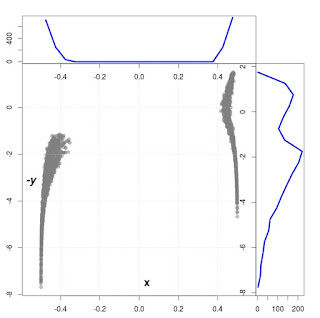
On all plots the dots are a result of numerical calculations of the Hamiltonian $H_{eff}$. Numerical simulations have been done for 30 GUE matrices $V$ with $N = 100$ and $M = 60$. Remaining values of parameters used for simulations:

1. energies: $E_{A} = -1/2$, $E_{B} = 1/2$,
2. number of states: for state $A$: $N_{A} = 50$, for state $B$: $N_{B}=50$,
3. interaction couplings are described for each plot separately.

At the beginning, for a comparison with existing models we shows on Fig. 2,3 and 4 a situation where $\gamma_{A} = \gamma_{B}$ and different values of $\gamma_{B}$. A similar plots one can find in the work [1].
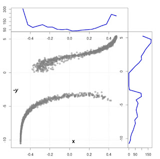
For a better visibility we used for scale $y$ logarithmic scale. In our case $y \leftarrow -log( \left| y \right| )$, so the value $y=-3$ corresponds to $y = 10^{-3}$.

Fig. 2. Simulation for $\gamma_{A} = \gamma_{B} = 0.0025$ in energy units. The left vertical plot shows the integrated density profile of the width of calculated eigenvalues. The upper picture presents the integrated spectral density showing the width of energy states.

Fig. 3. Simulation for $\gamma_{A} = \gamma_{B} = 0.01$. An creation of two timescales of the eigenvectors is visible.

Fig. 4. Simulation for $\gamma_{A} = \gamma_{B} = 0.5$.

















The next Figs (5,6,7 and 8) shows asymmetric situations where $\gamma_{A} = \gamma_{B}/10$ and different values of $\gamma_{B}$. Detailed values of other parameters are noted in the figure description.

Fig. 5. The situation with $\gamma_{B} = 0.01$ and $\gamma_{A} = \gamma_{B}/10$.

Fig. 6. The eigenvalue spectrum calculated for $\gamma_{B} = 0.05$ and $\gamma_{A} = \gamma_{B}/10$.

Fig. 7. The spectrum calculated for $\gamma_{B} = 0.1$ and $\gamma_{A} = \gamma_{B}/10$.

Fig. 8. The spectrum calculated for $\gamma_{B} = 0.5$ and $\gamma_{A} = \gamma_{B}/10$.

Conclusions

The landscape presented on all plots of eigenvalues of the Hamiltonian $H_{eff}$ is quite straightforward for those who are familiar with atomic physics, especially interactions of multi-level atomic transitions with resonant light. We see clear existence of so called coupled and uncoupled level (states) combinations . The increase of the coupling constant $\gamma_{A|B}$ leads to a creation of grouping of eigenvalues.
The eigenfunctions in the Hamiltonian can be formed in such a way that some combinations of levels cancel the interaction part with the environment - they are called uncoupled (or trapped) states. The number of such states is $N-M$.
Other level eigenfunctions are coupled with the environment's states - such an eigenfunction we call coupled (or un-trapped) states ($M$ decaying states). Populations of trapped states can survive longer time (smaller values of y) in comparison to the un-trapped states, where the populations is exchanged between coupled states by the interaction term proportional to $\sqrt{\gamma_{A|B}}$.
Let us try to translate this physical picture into a social language.

1. The coupled (un-trapped) states: configurations of members (eigenfunction) which change a common opinion (eigenvalue) faster due to the interaction with a noisy environment represented by a different set of environmental opinions. Such an exchange of opinion is proportional to the interaction strength $\gamma_{i}$ ($i=A|B$).
2. The uncoupled (trapped) states: ideally, such configurations of members (eigenfunction) which create a stable combinations of a group members. They do not interact with the environment.

If we define an opinion power as a parameter proportional to the number of eigenfunctions which share the same range of opinions we see that in steady-state conditions the opinion created by the trapped states (i.e. weakly coupled with the environment) has a greater power of persuasion than an opposite social group characterized by the un-trapped member's configurations (i.e. strongly coupled to the environment).
A higher level of noise (larger value of $\gamma_{A|B}$ and different values of couplings $\gamma_{A} < \gamma_{B}$) doesn't lead to reduction of a significance of unwanted opinions but creates just the opposite action:
it sharpens the polarization of existing opinions and increases the importance of resistance against the environment in a society. Such a situation can be well identified nowadays. The noisy environment is created by mainstream media. What one can find in such an environment: an increasing number of different subjects, news focused on accidents, preferred shorter forms and propagation of a number of opposite opinions and many other similar, as well as different ways of distraction of reader's attention.
Groups of people strongly coupled to such a media stream are not able to define a private opinion and they are easy to manipulate. It also means that the number of people in such a chaotic environment will migrate rather to more stable social groups (trapped states), not so strongly dominated by the mainstream news.
The creation of people without a strong, private opinions is a goal of the present liberal governments. But, as it is presented in this note the chosen way of social control leads just to opposite behaviour. You can see it around yourself, don't you ?
In the model, we used the condition where the number of intermediate states in the environment $M$ is smaller that the number of states in considered social groups $N$: $M < N$.
The opposite case leads to a bit different picture than described in this note, but it is a subject for an another post.


Bogdan Lobodzinski
Data Analytics For All Consulting Service

References:

1. E.Gudowska-Nowak, G. Papp and J. Brickmann, Two-Level System with Noise: Blue's Function Approach, Chem. Phys., 220 120-135 (1997)

Small and medium-size companies: any chance to grow in the Big Data dominated environment ?

Today I watched a video presenting European Truck Platooning Challenge 2016.
For those who are not familiar with the subject, it is about a test of self-driving trucks across Europe. The test was organized by the Dutch government. Main truck companies from Europe participated in running the event. You can watch the video here here and here.
It is a really great proof-of-concept project driven by the Big Data technologies.

However, in this note I don't like to write about details of the project. Instead, I would like to develop wider my first reflections after watching the video. I think everyone's conclusion will be that with this event all smaller transportation enterprises have got a Big problem. The problem can be verbalize by a question:
how to survive on the market dominated by big transportation players and their self-driving trucks across Europe ?
In the big transport companies the drivers will be replaced by the lawyers, but what about smaller transport businesses ?

Of course the problem is not only related to the transport industry. Similar situation appears in each branch of commerce. Therefore, the more general question, is:
how smaller enterprises can find themselves in the business environment dominated by the Big Data technologies governed by big parties ?
It is a bit similar to the competition between members inside a social group:
how to survive in a group dominated by set of rules profitable mainly for those who created those regulations.
Each of us can find clear example of such an environment from his own experience.

In my opinion, a possible solution of the problem can be found in a grouping of small companies into a fair-shared societies glued by common goals and business activity. Such a group has a bigger chance of survival than a single member, especially if all members can coordinate all individual actions, in such a way that only these processes which are profitable for the group and for the participant should be realized. It may sound like a socialism utopia - so it may mean - forget it, not possible for realization.

However, I am more and more convinced that such a procedure of business activity is possible if all human emotional behavior can be removed from a decision making processes. Remember, we are talking about methods to lead business in a most effective way. Such a decision creator can be realized by a Big Data driven decision making system using machine learning algorithms . If we have a group of a few enterprises and each company makes available his business data (like details of contacts, details of realized tasks and preferences, etc. ) for the decision-making system, a proper Big Data framework can create suggestions how to move forward using well established probabilities.
A client can look for a doer by communications with a group accessing the representative portal providing specification of task(s), or asking directly a chosen company.
In opposite, each group member can act fully autonomously, looking for customers individually or can use a group representative hints created by the decision-making system. In both cases the group representative framework acts as a Data driven decision creator:

1. for customer: suggesting proper companies from the group
2. for companies in the group: informing chosen entities about requested tasks.

The structure of the group reminds a bit the franchise business model. In contrary to a franchiser a group member don't have to follow any business concept and there is no need for any kind of standardizations in terms of provided services. The only payment which have to be provided by the group participants is a cost of the service and the development of a proper "Big Data"/Machine Learning infrastructure.

Summarizing this short note, the goal of described above business association is creation and support of strategies for sustainable growth of small sized enterprises in a Big Data dominated environment. The common features among all participating parties in the group should be community of the type of business activity and goals.

Unfortunately, details are usually much mode complicated, but my intention was to sketch a general picture of a structure with (in my opinion) a highest chance to become profitable in the Big Data business era.

I will appreciate any comment and opinion about the idea sketched above.


Bogdan Lobodzinski
Data Analytics For All Consulting Service

Recommender Systems and q-value Potts model

Introduction

Recommendation system (RS) can be described in a general way as a class of applications used to predict a set of items with highest probability of acceptance by a given user and is based on user's responses. The RS connects users with items and it is usually described from the point of view of the performance of algorithms used in the system.
In this note I would like to raise the following question: what can we learn by applying a q-valued Potts model to datasets created by recommender system ? The Potts model describes interaction of a set of spins distributed on a lattice. In contrary to Ising model, spins in the $q$-valued Potts formulation can take $q$ possible states (values).

Analysis

Let us consider a database created by a given RS where each item is characterized by a set $\{rating,tag\}$. Both, the $rating$ and $tag$ values are determined by independent users. From the $tag$ value one can extract a set of users who tagged the item. Those users make an $y$ coordinate. The $x$ coordinate is created by the users who made $rating$ instances. Both coordinates can be used for creation of $x-y$ lattice with $z$ values corresponding to the $rating$ variable.
It is obvious that the available items and users evolve with time in some way. Therefore it is not possible to determine close neighbours of a given spin placed in a lattice point $\{x,y\}$. In order to avoid this problem I assume that all spins on the lattice can interact with each other with the same coupling constant equal 1. After such assumptions the data can be described as the long-ranged $q$-value Potts model with parameter $q$ corresponding to the number of voting options. Using mathematical notations, for a given time $t$ we have $x-y$ lattice occupied by spins $\sigma_{i} = 1,..,q$ . The lattice (graph) state is described by the energy $E$ due to the interaction between spins $\sigma_{i}$: $$E = - \sum_{i,j} \delta_{\sigma_{i},\sigma_{j}}$$ and by the order parameter (also known as a magnetisation) $M$ defined as $$M = \frac{\left( q \max\{n_{i}\} - N \right)}{\left(q-1\right)} .$$ In the formulas above: $\delta$ is the Kronecker symbol, $N$ is the total number of spins in the lattice, $n_{i} <= N$ denotes the number of of spins with orientations $\sigma_{i}$.
Each graph is described by the per-graph quantities: $e = E/N$ and $m = M/N$ . The maximum order in a graph corresponds to $m = 1$ and is equivalent to all spins with the same orientation. The perfect disorder is specific for a case when all orientations are equally numerous: $\max\{n_{i}\} = N/q$, this state corresponds to $m = 0$. As a data for the model I used the movie dataset [1]. The database has 10 voting options ($q = 10$) with possible voting values $V = \{0.5,1,1.5,2,2.5,3,3.5,4,4.5,5\}$.
In the analysis, $y$ users (determined from $tag$ values) were selected globally for entire time range available in the data (9/17/1997 - 1/5/2009 ). The $x$ users were determined for each time step which was chosen as 1 day. For each time step I calculated the energy $e$ and the order parameter $m$. Details of calculations are available in R language listed in [2]. The calculations were performed for different numbers of voting options $q$ and available values $V$. Selected values of $q$ and $V$ are following

1. $q = 3$, $V = \{2, 3, 4 \}$
2. $q = 4$, $V = \{2, 3, 4, 5 \}$
3. $q = 5$, $V = \{1, 2, 3, 4, 5 \}$
4. $q = 6$, $V = \{1, 1.5, 2, 3, 3.5, 4\}$
5. $q = 7$, $V = \{1, 1.5, 2, 2.5, 3, 3.5, 4\}$
6. $q = 10$, $V = \{0.5, 1, 1.5, 2, 2.5, 3, 3.5, 4, 4.5, 5\}$

For each subset defined by $q$ I made an averaging fit of calculated time evolution of variables $e$ and $m$ using local polynomial regression fitting smoothing (loess) with parameters [3]:

loess(y ~ x, family="gaussian", span=.75, degree=1)

All results are presented on plots below (the R source code for plots is listed in [3]). The energy $e$ (normalized to the same initial value) shows a behaviour typical for the Potts model:
But the most unexpected time evolution is seen on plot of the order parameter $m$:
The relaxation of the order parameter $m$ shows a two-staged process, well distinguished for $q < 6$ . The same behaviour is also visible for $q >=6$ however the steady-state value is not reached by the system yet. The final value of the order parameter also depends on the number of voting options. The stable value of $m$ parameter is higher for models with $q < 6$ ($\approx 0.6$) than for $q >=6$ ($\approx 0.4$). But this result should be checked more carefully on other datasets and it is too early to conclude this observation.

Conclusions

After some analysis work with the dataset from the RS, let me gather 2 main points:

1. two-staged relaxation process of the order parameter $m$ could be related to the different dynamical mechanisms. One of them leads to the exponential decay and the second one to the self-organizing phenomena. In terms of users behaviour, it suggests existence of two classes of users: randomly using the RS which could be responsible for the fast decay of the parameter $m$ and visitors of the RS with more stable opinions about voting subject. The stabilizing effects due to the non-random visitors will be specific rather for longer working rating webpages. Due to this feature I expect different performance of the same RS on a newly created rating website and on the rating site working for longer time .
2. The time scale of the order parameter $m$ decay after which the stable stage is reached is faster for smaller $q$ parameter. For the dataset used for the analysis the decays can be grouped for models with $q < 6$ and $q >=6$. This observation implies that a better performance of RS can be achieved for a system with smaller number of voting options.

Any comments and opinions greatly appreciated, thanks.


Bogdan Lobodzinski

Data Analytics For All consulting Service

References

[1] As a data for the model I used the movie dataset created by:

• [url=http://www.grouplens.org]Movielens from GroupLens research group[/url],
• [url=http://www.imdb.com]IMDb website[/url],
• [url=http://www.rottentomatoes.com] Rotten Tomatoes website[/url],

build by Ivan Cantador with the collaboration of Alejandro Bellogin and Ignacio Fernandez-Tobias, members of the Information Retrieval group at Universidad Autonoma de Madrid. The data can be downloaded from http://ir.ii.uam.es/hetrec2011//datasets.html site. [2] the source code in R for calculation of energy $e$ and order parameter $m$ for 4 voting options ($q = 4$) with available values $V = \{2,3,4,5\}$.

// Code
library(readr)
library(rgl)
library(MASS)
library(reshape2)

# Set a random seed for reproducibility
set.seed(1)

# set the q value of the model
q0 <- 4
# set the value options:
options <- c(2,3,4,5)
# set the file name with output:
Output <- "Params_q4.csv" 

cat("reading the data\n")
prefix <- "../moviedata/"
user_rated_input <- paste0(prefix,"user_ratedmovies.dat")
userrate<- read.table(user_rated_input, header=TRUE)

user_tagged_input <- paste0(prefix,"user_taggedmovies.dat")
usertag <- read.table(user_tagged_input, header=TRUE)

cat("Data manipulation\n") 

# 1. replace time by secs
userrate$timeinDays <- as.numeric(as.POSIXlt(userrate$time, format="%m/%d/%Y"))
usertag$timeinDays <- as.numeric(as.POSIXlt(usertag$time, format="%m/%d/%Y"))

# 2. rearrange data first in descending time order:
sort.userrate <- userrate[order(userrate$timeinHours) , ]
sort.usertag <- usertag[order(usertag$timeinDays) , ]

GetMatrix <- function(inputX,inputY, inputZ) {
        x <- NULL
        y <- NULL
        z <- NULL
        x <- inputX
        y <- inputY
        z <- inputZ
        
        # check duplications:
        d1<-NULL
        d1<-data.frame(x,y)
        indexes<-NULL
        indexes<-which(duplicated(d1))
        if (length(indexes)) {
                d1<-d1[!duplicated(d1),]
                z<-z[-indexes]
        }
        mydf <- NULL
        mydf <- data.frame(d1,z)
        mat <- NULL
        mat<-as.matrix(acast(mydf, x~y, value.var="z"))
        mat[is.na(mat)] <- 0
        mat
}

lowerLimit <- q0

EnergyAv <- NULL
MagAv <- NULL
items <- NULL 

for (item in unique(sort.userrate$time)) {  # <- Day's timescale                
                tx <- NULL
                tx <- subset(data.frame(sort.userrate),time == item)

                if ( min(dim(tx)) > 0 ) {
                   merged <- NULL                        
                   merged<-merge(tx,sort.usertag,by=c("movieID"))                
                   if (min(dim(merged)) > 0 ) {
                      myMat <- NULL
                      myMat <- GetMatrix(merged$userID.x,merged$userIDy,merged$rating)
                      myMat1<-NULL
                      myMat1<-myMat[!(myMat == 0)]

                      # selection of states:2,3,4,5 for q = 4 valued model:
        myMat1 <- myMat1[myMat1 %in% options]
               nrOfSpins <- length(myMat1)
        if ( (nrOfSpins > lowerLimit) ) {
     # Energy: 
                          Energy <- 0
                          # counting nr of pairs:
                          for (elem in table(myMat1)) {
                               Energy <- Energy -(choose(elem, 2))
                          }
                          EnergyAv <- c(EnergyAv,Energy/nrOfSpins)
                                        
     # Order parameter Mag:       
                          Mag <- 0
                          Mag <- (q0*max(table(myMat1))-nrOfSpins)/(q0-1)
                          MagAv <- c(MagAv, Mag/nrOfSpins)
                                 
                   # time:
                          items <- c(items, item)
                      }
                   }        
                }
}

cat("Saving results ...\n")
dfq<-NULL
dfq<-data.frame(Time=items,Mag=MagAv,En=EnergyAv)
write_csv(dfq, Output )

[3] R source code used for creation of the plots:

// Code
library(readr)
require(ggplot2)
library(rgl)
library(MASS)
library(lattice)

# read data
prefix <- "./"
q3_input <- paste0(prefix,"Params_q3.csv")
q4_input <- paste0(prefix,"Params_q4.csv")
q5_input <- paste0(prefix,"Params_q5.csv")
q6_input <- paste0(prefix,"Params_q6.csv")
q7_input <- paste0(prefix,"Params_q7.csv")
q10_input <- paste0(prefix,"Params_q10.csv")

q3 <- read.table(q3_input, sep=",", header=TRUE)
q4 <- read.table(q4_input, sep=",", header=TRUE)
q5 <- read.table(q5_input, sep=",", header=TRUE)
q6 <- read.table(q6_input, sep=",", header=TRUE)
q7 <- read.table(q7_input, sep=",", header=TRUE)
q10 <- read.table(q10_input, sep=",", header=TRUE)

# fits & plots:
elems <- list(q3,q4,q5,q6,q7,q10)

# fit of the order parameter:
myx1 <- NULL
mypred1 <- NULL

for (ind in 1:length(elems)) {
        tmp <- NULL
        tmp <- data.frame(elems[ind])

        x <- as.numeric(as.POSIXlt(tmp$Time, format="%m/%d/%Y"))
        myx1 <- c(myx1,list(x))
        
        y <- with(tmp, Mag)
        eval.length <- dim(tmp)[1]
        fit.loess2= loess(y ~ x, family="gaussian", span=.75, degree=1)
        
        pred <- predict(fit.loess2, data.frame(x=x))
        fac<-1/pred[1]
        pred <- pred*fac
        mypred1<- c(mypred1,list(pred))
}

# energy:
# fit of the energy parameter:
myx2 <- NULL
mypred2 <- NULL

for (ind in 1:length(elems)) {
        tmp <- NULL
        tmp <- data.frame(elems[ind])
        
        x <- as.numeric(as.POSIXlt(tmp$Time, format="%m/%d/%Y"))
        myx2 <- c(myx,list(x))
        
        y <- with(tmp, En)
        eval.length <- dim(tmp)[1]
        fit.loess2= loess(y ~ x, family="gaussian", span=.75, degree=1)
        
        pred <- predict(fit.loess2, data.frame(x=x))
        fac<-abs(1/pred[1])
        pred <- pred*fac
        mypred2<- c(mypred2,list(pred))
}

# plots:
xpos <- c(8.94,8.99,9.04,9.09) # x axis: log10(time) position
x01 <- log10(myx1[[1]])
origin_date <- "1970-01-01"
t1 <- substr(as.POSIXct(10^(x01[which.min(abs(x01-xpos[1]))]), origin = origin_date),1,10)
t2 <- substr(as.POSIXct(10^(x01[which.min(abs(x01-xpos[2]))]), origin = origin_date),1,10)
t3 <- substr(as.POSIXct(10^(x01[which.min(abs(x01-xpos[3]))]), origin = origin_date),1,10)
t4 <- substr(as.POSIXct(10^(x01[which.min(abs(x01-xpos[4]))]), origin = origin_date),1,10)
TimeLabels <- c(t1,t2,t3,t4)

colors <- terrain.colors(6)

plot(log10(myx1[[ind]]), mypred1[[ind]],type="l",lwd=6, col = colors[ind], xlab = "Log10(Time)", 
     ylab = "Normalized Order parameter", 
     ylim=c(0.2,1.0), xaxt = "n" )
for (i in seq(ind-1,1,-1)) {
        lines(log10(myx1[[i]]), mypred1[[i]],lwd=6, col = colors[i], xlab = "Time (s)", 
        ylab = "Counts")
}
legend("topright", inset=.05, title="q-values:",c("3","4","5","6","7","10"), fill=colors[1:6], 
horiz=TRUE)
axis(side = 1, at = xpos, labels = TimeLabels)#, tck=-.05)

# energy:
plot(log10(myx2[[1]]), mypred2[[1]],type="l",lwd=6, col = colors[1], xlab = "Log10(Time)", 
     ylab = "Normalized Energy", xaxt = "n")#, ylim=c(-,1.0) )
for (i in seq(2,ind,1)) {
        lines(log10(myx2[[i]]), mypred2[[i]],lwd=6, col = colors[i], xlab = "Time (s)", 
        ylab = "Counts")
}
legend("bottomleft", inset=.05, title="q-values:",c("3","4","5","6","7","10"), fill=colors[1:6], 
horiz=TRUE)
axis(side = 1, at = xpos, labels = TimeLabels)#, tck=-.05)

How Data Analytics can help small companies ?

Trying to operate on the market of micro, small and medium-sized enterprises as a data analyst serving solutions based on the machine learning techniques, I have to say - it is a difficult business.

In my opinion, the difficulties arise due to two main, entangled reasons:

1. completely missing knowledge about a potential of data analytics. Most company owners don't even accept a though that someone from outside of the firm can suggest how to improve his business productivity,
2. if someone sees the need of a data analytics, the second problem appears: it is the cost of such a project. It can be a serious problem if it is seen as a single payment without noticing a new business landscape which gets opened by the results of the data analysis.

Let us start with the second point: data analytics project costs.

First of all, a usual thinking is that a data analytics requires enormously complex hardware and software infrastructure, therefore it will cost much too much. The truth is just the opposite. All tools which are needed for data analytics tasks of small companies can be completed during a few working days without spending a penny. Actually, it is not fully true, you have to have a good, powerful notebook with access to the network. Already having a computer, what else do you need at the beginning ?

1. Linux as a free operational system, and software:
2. Python or/and R (in this case also Rstudio).

All of the above is available for free and downloadable from the Internet as an open source software. The most important part of the whole collection is your business database. Again, even if you collect data using commercial software specific for your activity, it is possible to convert most of the available formats into more accessible ones for the R or Python form. Sometimes, that work might require some effort but in general it is doable.
More problematic is the situation when the company data are on the paper only. What to do in such a case ?
Maybe your accountant can help somehow - in communication with the tax office some forms of digital data have to be used anyway.
Another solution is to initialize the data gathering from the scratch. It can be realized using open source databases installed on a cloud. The cloud is not a free choice but the management costs are really negligible if one compares the cost of cloud computing and storage with other business expenses. In case of a cloud usage, we have to add a note about security of your data, especially in terms of unauthorized external access to your data. Solution is very simple: the data analysis doesn't need real values in your database entries.
It is enough to replace, for example, real addresses of the company clients by short unique strings. Similar encryption can be done with numbers, using a common factor for all values in a given row. The real meaning of the unique strings and numerical factors remains in a company's hands.
If needed, one can use already existing datasets available for free.

Now, we get to the point where a data expert becomes a crucial person. The data scientist can merge the entrepreneur business knowledge with mathematics and practical machine learning solutions. This can lead to a better understanding of your business experience. But the final move belongs to the company managers, data analytics would lead to nothing if the results were not introduced into practical realizations.

Work of the data expert(s), usually includes

1. consultations: when points like these are discussed:
   • what the company would like to develop, explain, understand or predict,
   • availability of business data and how they are compatible with the company's goal,
   • preparation of a concluding question e.g. the final goal of the data analysis,
2. pilot solution: a creation of a test model which can be validated on the existing data and tested on a new set of data,
3. final realization: preparation of software tools which can be used on demand in daily business operations or on a regular basis using old and newly created data.

Between the lines written above a number of interactive actions is included where all obstacles or unpredicted behaviours are discussed. All that is performed until the desired result is achieved. The usual working time of the expert can be estimated between 50 hours (a week) for a micro projects up to several hundreds hours of work.

Now, one can ask how much data analytics products per working hour might cost ? The hourly rate can be estimated as 30 - 100 Euros. So, the final cost can vary between 1500 - 50000 Euro and more.

How to measure the efficiency of a data analytics project ?
A research performed by D. Barton and D. Court which was based on 165 large publicly traded firms shows that Data-driven decision-making can increase the output and productivity by 3-5% beyond the traditional improvement steps (Dominic Barton and David Court, Making advanced analytics work for you, Harvard Business Review, October 2012, Volume 90, Number 10, pp. 78–83). Using this estimation and assuming the smallest increase of 3% of a company output, a minimum enterprise outcome would be about 50 000 Euro for full recompensation of a smallest Data analytics project cost.

We treat the subject very generally, therefore some company owners will not be convinced why they should start to use data-driven decisions instead of relaying on the well grounded on the experience intuition . The numbers: 3-5% of outcome increase (set by the classical actions estimated by authors in cited above research paper) seem to be too small to be used as a solid argument in a discussion with small-firm owners.

Yet, let me add a few arguments which, I hope, can change a bit the dominated view of data analytics in small business.

1. The most important step: collection of data, especially in small companies is difficult due to the lack of knowledge and free manpower. However, that issue can be easily automated and (what is not negligible) the tool can be fully owned by the company. Collecting sufficient amounts of data takes time, it could be a quite long process in case of small-firm segments. Therefore, the sooner the data collection process will start, the sooner analytical process will become beneficial.
2. The data-driven management system requires more formalized and structured approach. It could be a difficult point in the transformation to the data-driven manner. But by answering simple questions (sometimes completely neglected and treated as a not important at all) one can achieve the biggest goals. Just a few examples of questions:
   Who is buying a given flavour of a bread ?
   How is the buying of bread correlated with time ?
   Which cookies prefer young, mature and older customers ? etc.
   All these answers can be provided by data analytics. And it is straightforward to notice that knowing the answers and following them in real world means clearly higher revenue.
   
3. What if the results of data analytics are consistent with the firm-owner intuition ? In our opinion it is a wrong question: even if data-driven development suggestions are compatible with the well established experience of the company leader, we are talking about specific numbers: how many cookies should be delivered to the shop, how many breads should be produced, etc. Do you believe that any, even the best intuition would provide the same numbers ?. Obviously not. Therefore, the initial question should be replaced by the statement: The data-driven results are capable to increase assurance of the manager's intuition.
   
4. and finally the non BigData conclusion: new technologies in a company business opens the firm to new ideas and tedious work becomes more interesting.

So, what do you think Dear Reader ? Are you ready for innovations in your view of the company's management style ?

Bogdan Lobodzinski
Data Analytics For All Consulting Service